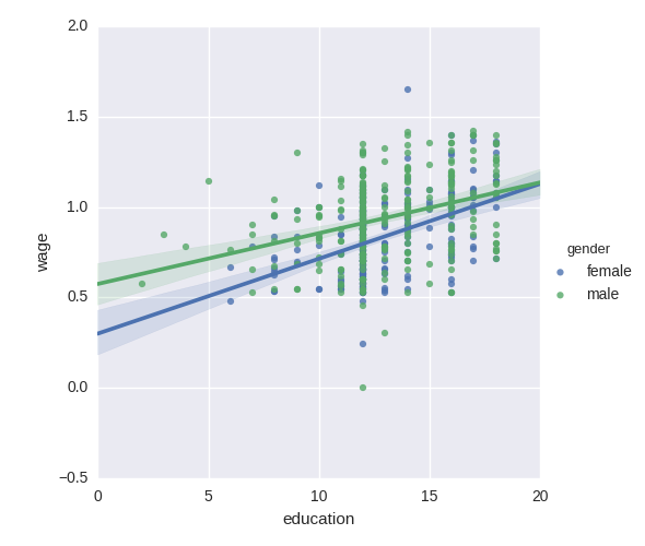
Wages depend mostly on education. Here we investigate how this dependence is related to gender: not only does gender create an offset in wages, it also seems that wages increase more with education for males than females.
Does our data support this last hypothesis? We will test this using statsmodels’ formulas (http://statsmodels.sourceforge.net/stable/example_formulas.html).
Script output:
  OLS Regression Results
==============================================================================
Dep. Variable:                   wage   R-squared:                       0.193
Model:                            OLS   Adj. R-squared:                  0.190
Method:                 Least Squares   F-statistic:                     63.42
Date:                Mon, 21 Sep 2015   Prob (F-statistic):           2.01e-25
Time:                        19:08:36   Log-Likelihood:                 86.654
No. Observations:                 534   AIC:                            -167.3
Df Residuals:                     531   BIC:                            -154.5
Df Model:                           2
==================================================================================
                     coef    std err          t      P>|t|      [95.0% Conf. Int.]
----------------------------------------------------------------------------------
Intercept          0.4053      0.046      8.732      0.000         0.314     0.496
gender[T.male]     0.1008      0.018      5.625      0.000         0.066     0.136
education          0.0334      0.003      9.768      0.000         0.027     0.040
==============================================================================
Omnibus:                        4.675   Durbin-Watson:                   1.792
Prob(Omnibus):                  0.097   Jarque-Bera (JB):                4.876
Skew:                          -0.147   Prob(JB):                       0.0873
Kurtosis:                       3.365   Cond. No.                         69.7
==============================================================================
                            OLS Regression Results
==============================================================================
Dep. Variable:                   wage   R-squared:                       0.198
Model:                            OLS   Adj. R-squared:                  0.194
Method:                 Least Squares   F-statistic:                     43.72
Date:                Mon, 21 Sep 2015   Prob (F-statistic):           2.94e-25
Time:                        19:08:36   Log-Likelihood:                 88.503
No. Observations:                 534   AIC:                            -169.0
Df Residuals:                     530   BIC:                            -151.9
Df Model:                           3
============================================================================================
                               coef    std err          t      P>|t|      [95.0% Conf. Int.]
--------------------------------------------------------------------------------------------
Intercept                    0.2998      0.072      4.173      0.000         0.159     0.441
gender[T.male]               0.2750      0.093      2.972      0.003         0.093     0.457
education                    0.0415      0.005      7.647      0.000         0.031     0.052
education:gender[T.male]    -0.0134      0.007     -1.919      0.056        -0.027     0.000
==============================================================================
Omnibus:                        4.838   Durbin-Watson:                   1.825
Prob(Omnibus):                  0.089   Jarque-Bera (JB):                5.000
Skew:                          -0.156   Prob(JB):                       0.0821
Kurtosis:                       3.356   Cond. No.                         194.
==============================================================================
Python source code: plot_wage_education_gender.py
##############################################################################
# Load and massage the data
import pandas

import urllib
import os

if not os.path.exists('wages.txt'):
    # Download the file if it is not present
    urllib.urlretrieve('http://lib.stat.cmu.edu/datasets/CPS_85_Wages',
                       'wages.txt')

# EDUCATION: Number of years of education
# SEX: 1=Female, 0=Male
# WAGE: Wage (dollars per hour)
data = pandas.read_csv('wages.txt', skiprows=27, skipfooter=6, sep=None,
                       header=None, names=['education', 'gender', 'wage'],
                       usecols=[0, 2, 5],
                       )

# Convert genders to strings (this is particulary useful so that the
# statsmodels formulas detects that gender is a categorical variable)
import numpy as np
data['gender'] = np.choose(data.gender, ['male', 'female'])

# Log-transform the wages, because they typically are increased with
# multiplicative factors
data['wage'] = np.log10(data['wage'])


##############################################################################
# simple plotting
import seaborn

# Plot 2 linear fits for male and female.
seaborn.lmplot(y='wage', x='education', hue='gender', data=data)


##############################################################################
# statistical analysis
import statsmodels.formula.api as sm

# Note that this model is not the plot displayed above: it is one
# joined model for male and female, not separate models for male and
# female. The reason is that a single model enables statistical testing
result = sm.ols(formula='wage ~ education + gender', data=data).fit()
print(result.summary())

# The plots above highlight that there is not only a different offset in
# wage but also a different slope

# We need to model this using an interaction
result = sm.ols(formula='wage ~ education + gender + education * gender',
                data=data).fit()
print(result.summary())


# Looking at the p-value of the interaction of gender and education, the
# data does not support the hypothesis that education benefits males
# more than female (p-value > 0.05).


import matplotlib.pyplot as plt
plt.show()
Total running time of the example: 0.35 seconds ( 0 minutes 0.35 seconds)
